Project 4
By Alex Becker
In this project, the end goal is to create image mosaics by stitching together multiple images such that it just looks like one larger image, with no noticeable artifacts where the images are stitched together. We can achieve this by first obtaining the transformation to project one image onto the plane of another image. Then, we need to somehow blend the region where the images overlap, otherwise there will be noticeable edges between them, as there will be slight differences in the conditions of the two photographs.
Part A
1. Shooting the Pictures
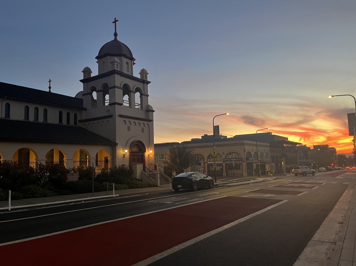
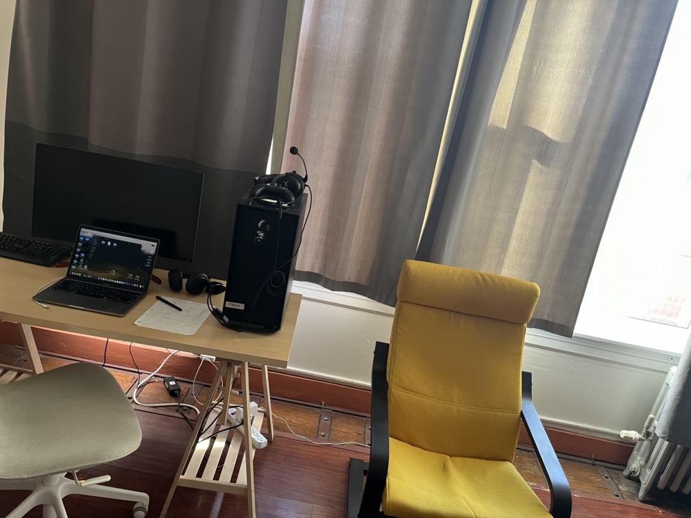
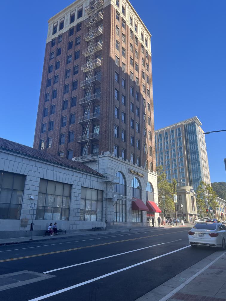
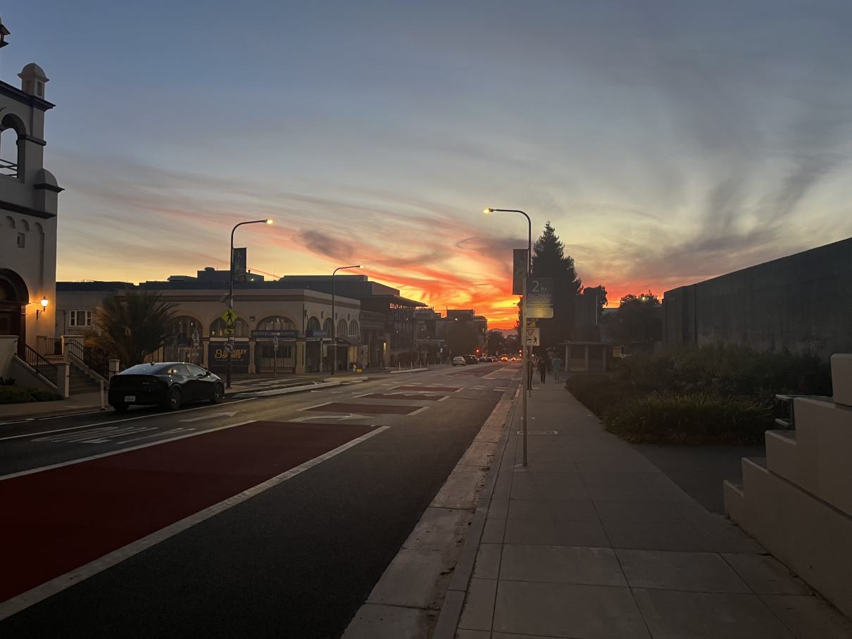
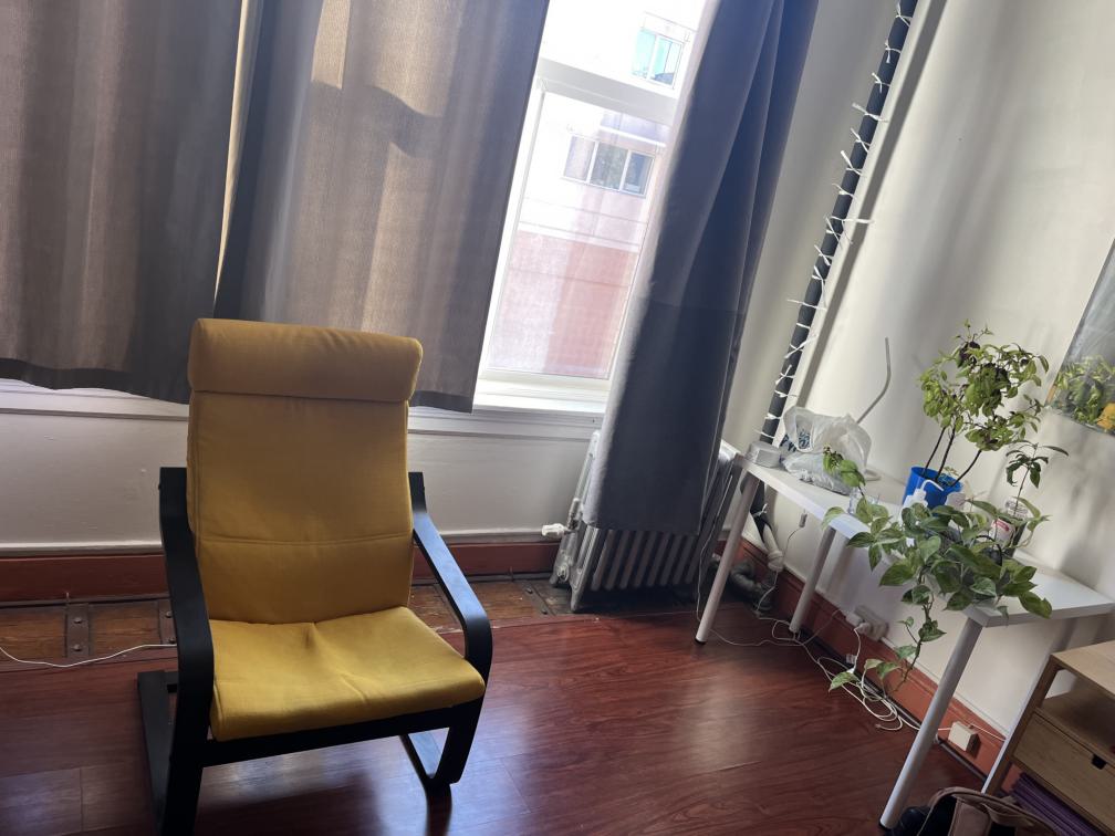
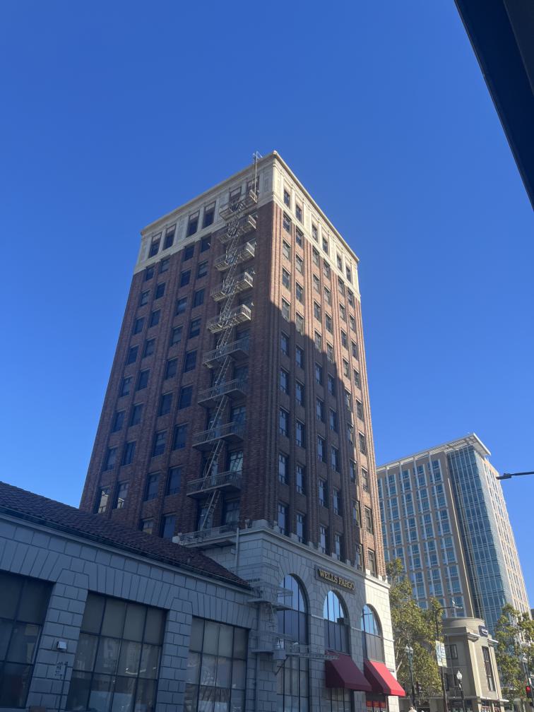
Below are the the images that I wanted to use to create 3 different mosaics.
Recovering Homographies
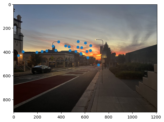
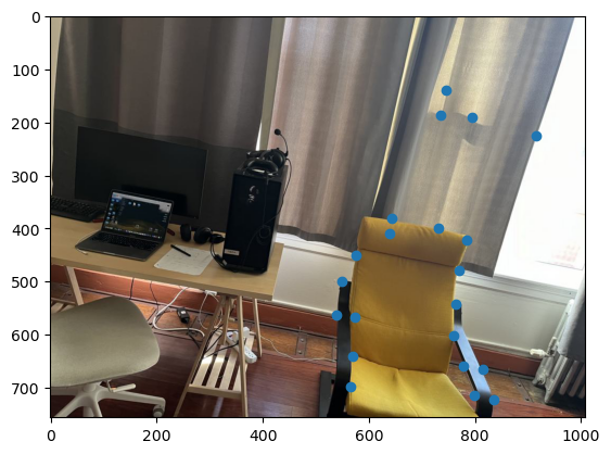
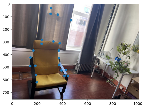
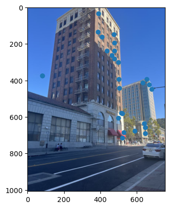
Now for each pair of images that will make one mosaic, we need to find the correct transformation to project one image onto the plane of the other. The type of transformation we want is a homography, which has 8 degrees of freedom meaning we can recover the homography matrix if we have 4 sets of corresponding points between the two images.
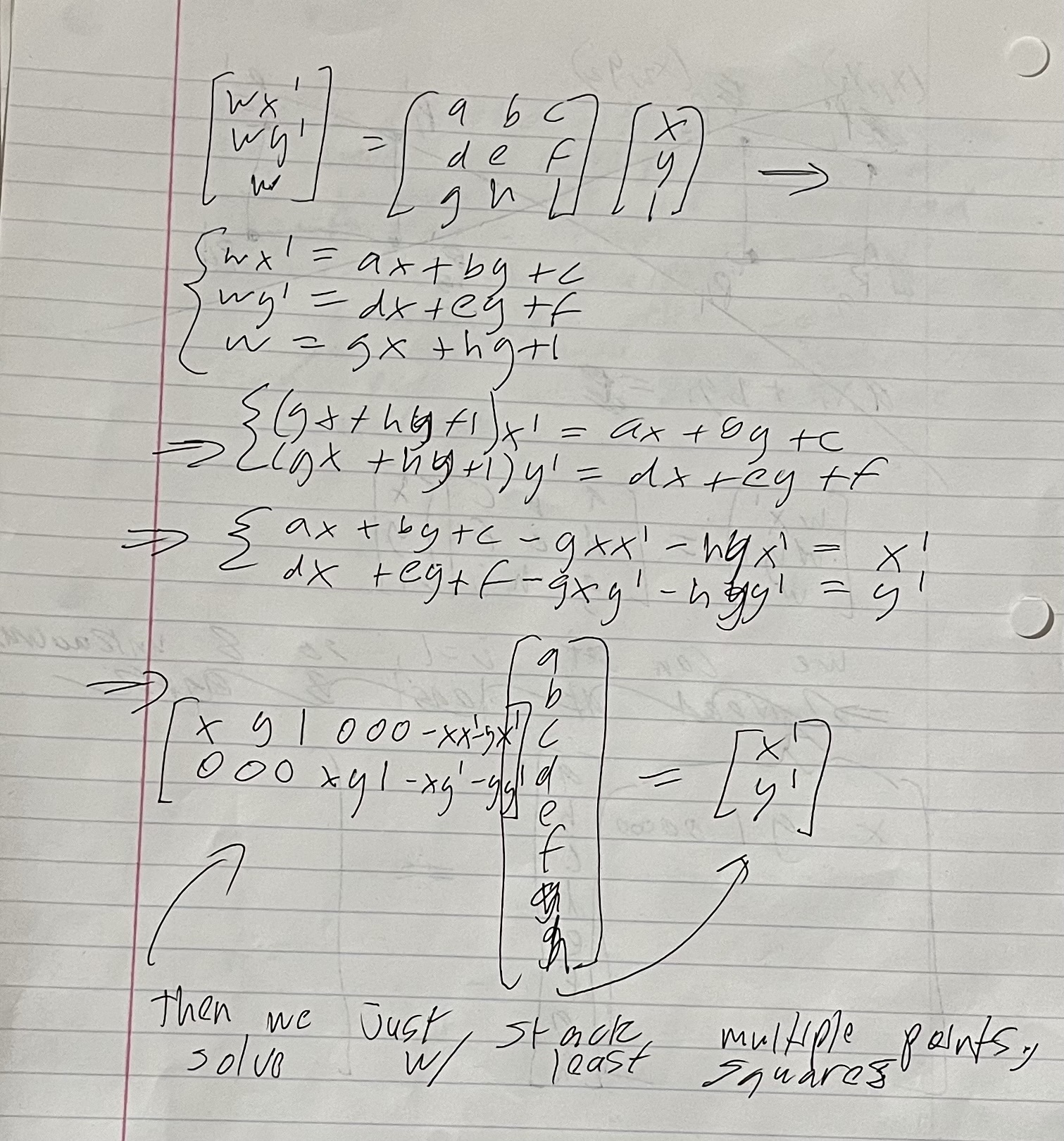
In the work above, we first see how we transform point (x, y) with a homography matrix to get point (x’, y’), the corresponding point in the other image. However, we use homeogeneous coordinates so we have to divide (wx’, wy’, w) by w after the transformation to get the point in 2D coordinates. Then we can see that if we want to determine the 8 parameters needed to determine the homography (last equation), we can just use 3 additional correspondences in addition to the one already shown, and stack corresponding rows on the left matrix and right vector. Then, we can just directly solve for the parameters. However, in reality it makes more sense to use more than 4 correspondences, as the manually chosen ones will not be perfect and can lead to an unstable homography. If we select more points, we stack as we did previously but then use least squares to get an estimated solution.
Warping the images
Now, we can compute the needed homography for all of the mosaics, but we still need to actually apply the transformation and ensure that the final image is the correct size so that it will contain the full mosaic. We also have the option of doing forward warping or inverse warping. I chose to do inverse warping since I knew how to implement it from the previous project, and it prevents having holes in our warped image. To ensure that the full mosaic would be in the final image, I wrote a function to compute the size of the final bounding box. I did this by just warping the corners of the image to be transformed, and then finding the size of the box that would enclose this projected image along with the image it’s being projected onto. I also had to ensure that the top left corner of the bounding box was treated as (0,0) so that the images would be properly overlayed after the transformation. For the warping, I performed inverse warping across all 3 color channels, using interpolation to get the correct pixel values.
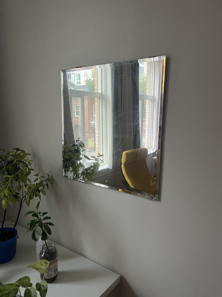
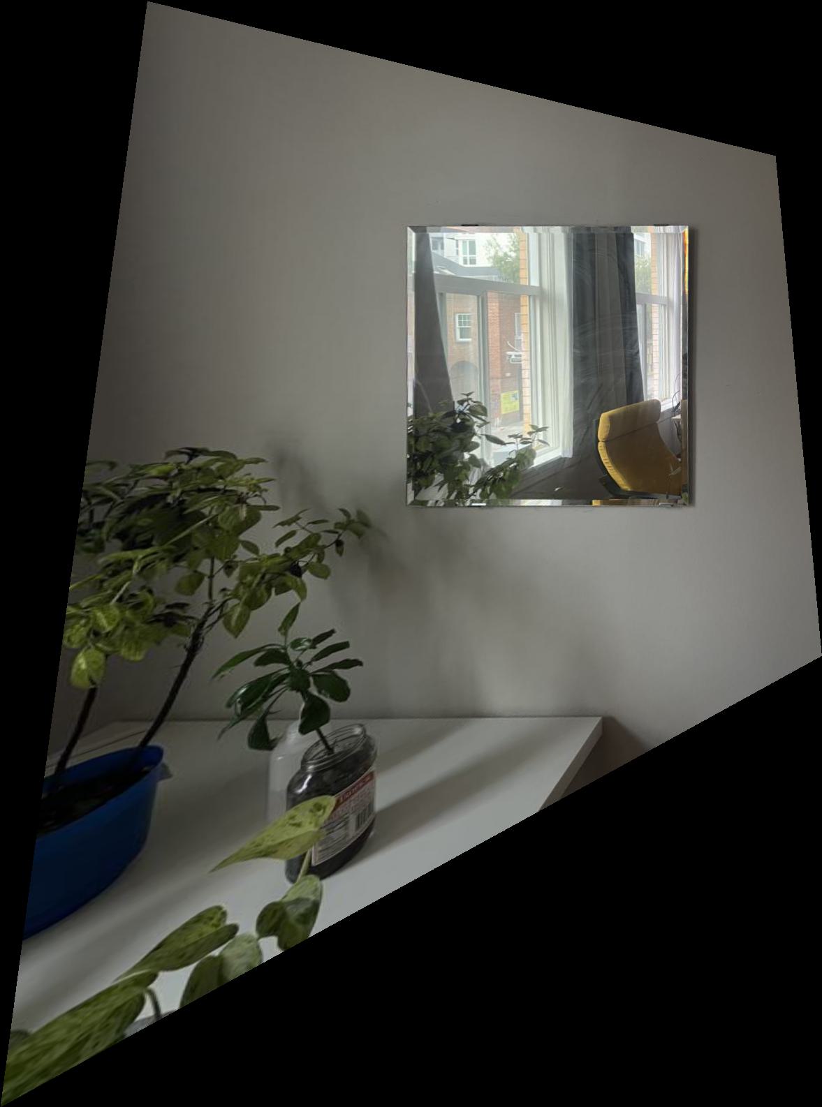
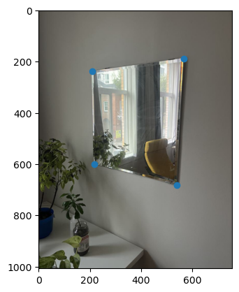
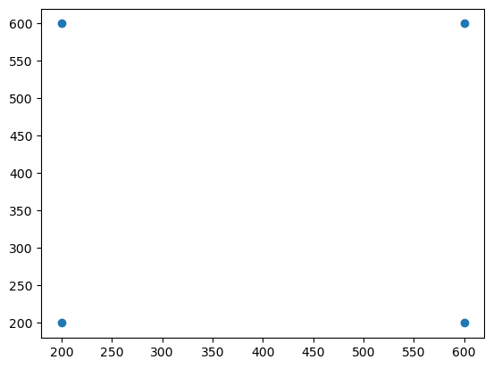
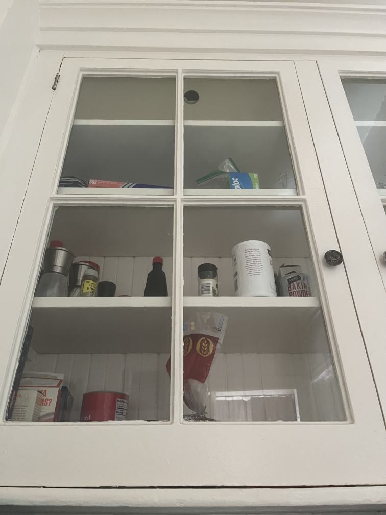
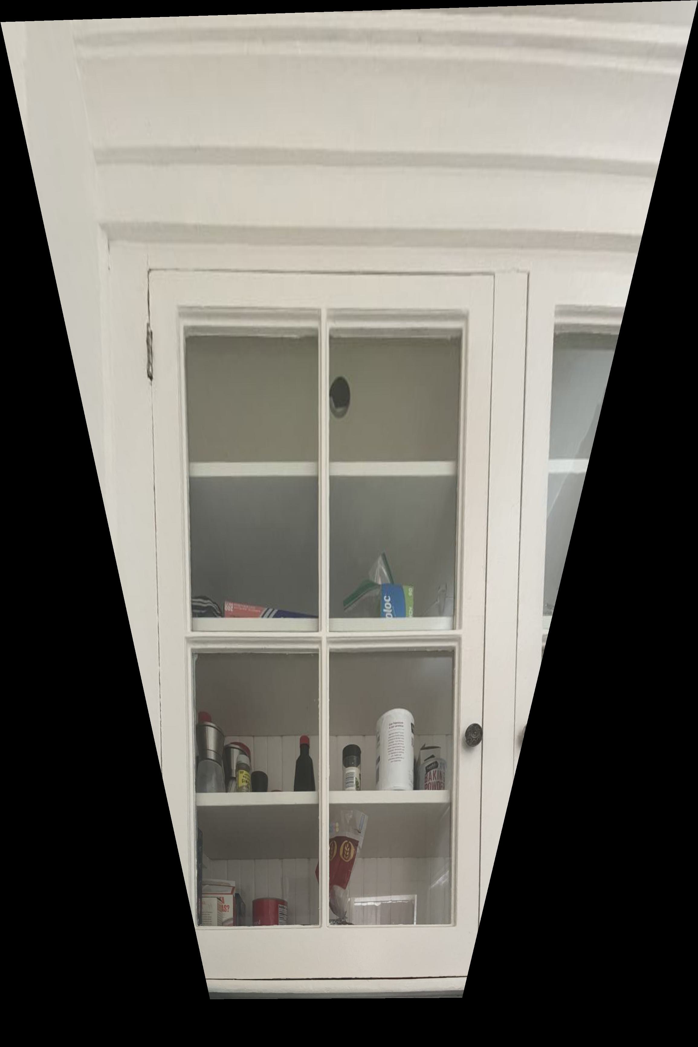
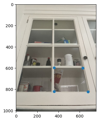
First, to test my warping, I used it on the two images below. I wanted to rectify the images so that we see the view of looking directly at them. I did this by using objects with known shapes, so that the correspondences would be easy to choose. Below are the rectifications and correspondences.
Blend Images into a Mosaic
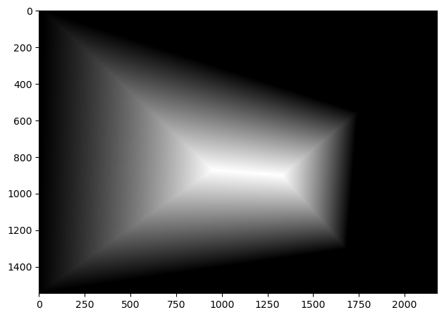
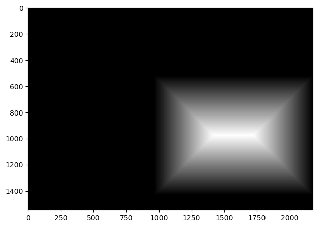
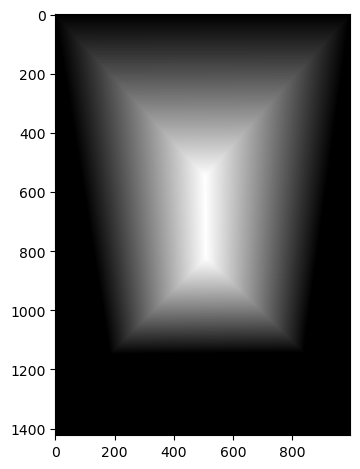
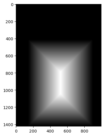
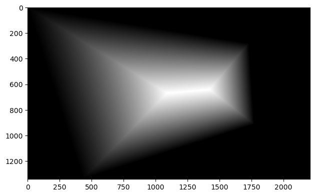
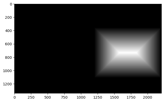
Now that we have the warping working, we can actually create the mosaics as described earlier. However, we also need to blend the images together well. For this, I used two band blending, where I high and low passed the images, applying different blending methods to each of the frequency bands. In particular, I created masks for each image, where the value of each pixel in the mask is the distance to the closest edge. Then I normalize the masks so that the highest value is 1. For the high frequencies, the values in the resulting mosaic were taken from whichever image’s mask has a higher value at that location. For the low frequencies, I used the masks again, but this time used the mask values in a weighted average of pixel values. Below are the resulting mosaics as well as the masks.


Part B
In part B of the project, the goal is to create these mosaics automatically given input images, meaning we will no longer have to manually select correspondences as we did before. To achieve this, we use techniques described in the paper Multi-Image Matching using Multi-Scale Oriented Patches by Brown et al.
Detecting Corner Features
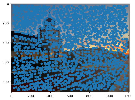
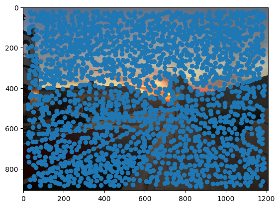
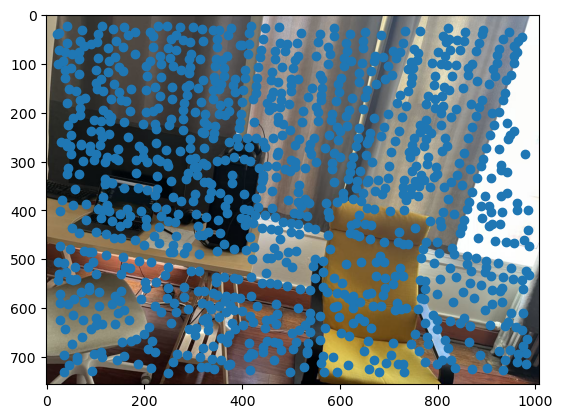
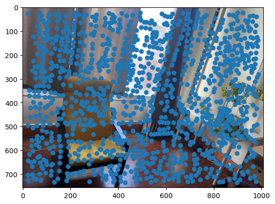
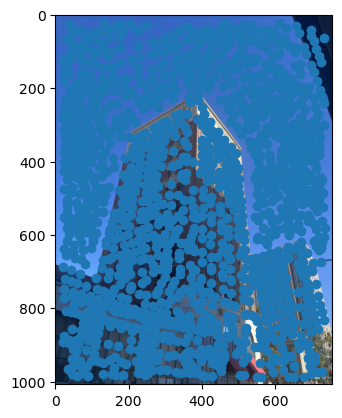
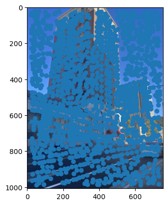
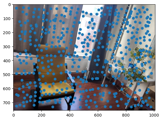
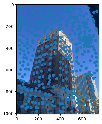
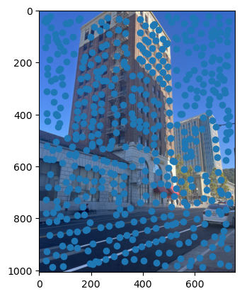
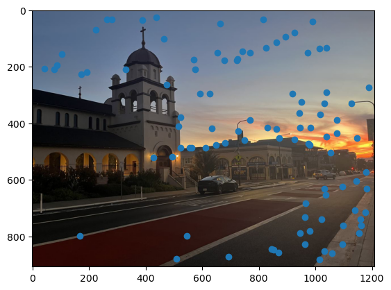
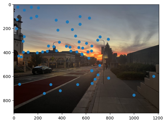
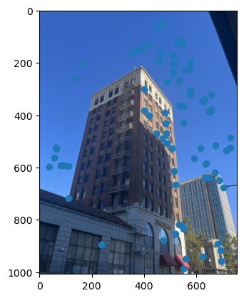
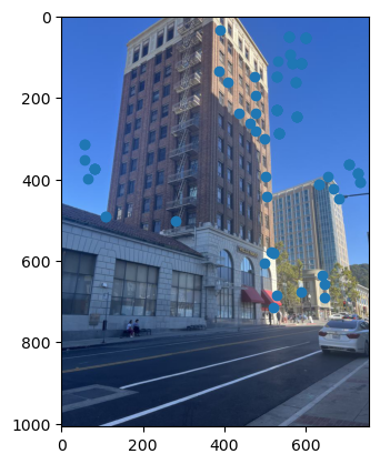
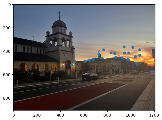
First, we need a way to automatically detect corner features, since we are no longer manually selecting them. One strategy to achieve this is to use Harris interest point detection, described in section 2 of the paper. Basically, this method will identify “corners,” which are locations in the image where if we have a window around that point and move it, there will be a large change in L2 distance between the original and shifted images, no matter which direction we shift the image. This makes sense as that’s essentially what a human definition of a corner is. However, the features detected will not always look like corners to us. Below are the detected corners for each set of images.
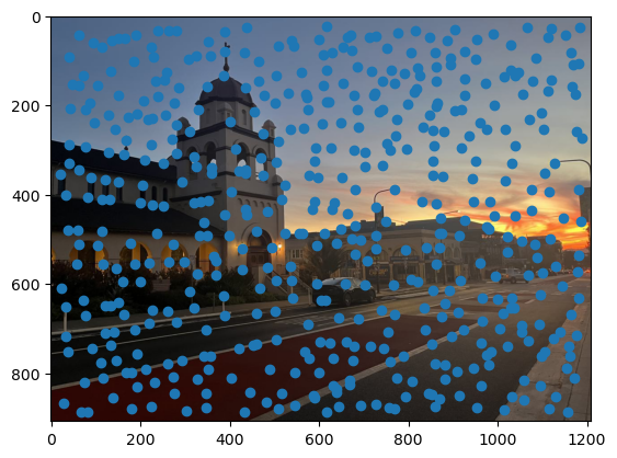
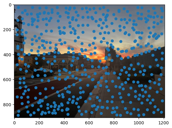
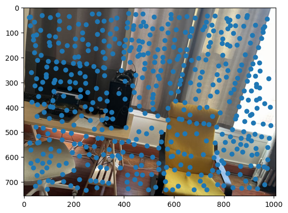
As you can see, we get many resulting Harris corners, about 2000 per image in my case. There’s no reason that we need this many correspondences, as in the manual one we only used about 20. Additionally, we don’t actually have correspondences yet, just a set of points from each image. In order to reduce the number of detected corners, we use Adaptive Non-Maximal Suppression, also described in the paper. With this technique, we want to suppress or eliminate many of the corners, particularly ones that are not as strong. Fortunately, the Harris method provides us with a score for each detected corner that gives us an idea of the corner strength. However, if we were just to keep the points with the top 500 scores for example, the points would most likely be clustered in parts of the image where there are a lot of obvious corners, for example on the building above. However, we want the points to be distributed uniformly across the images to ensure that we have enough points where the images have overlapping content. Otherwise, there wouldn’t actually be points we could use as correspondences. ANMS is the solution to this, and it works by computing a minimum suppression radius for each point, which is just the distance to the closest point that has a score above a certain threshold. For example, in my case the score of the other point times .9 had to be greater than the considered point for it to determine its radius. Once we compute these radii, where the strongest point has an infinite radius, we can just take the 500 points with the highest radii, and these will be better distributed. Below are the selected points for each set of images after running ANMS.
Extracting Feature Descriptors for each feature point
and Matching the Feature Descriptors
Now, we have reduced the number of points while maintaining a uniform distribution, but we still don’t have correspondences. Therefore, we need to match the features between the two images in each pair. To do this, we essentially take a window around each feature and try to find a matching window around a feature in the other image. If no matching window is found, we discard that point, as it could be unique to the image. Specifically, I took a 40x40 pixel patch around each point in one image, and then downscaled it with anti-aliasing to an 8x8 patch. This is done to essentially low-pass the patch since we don’t want high frequencies, which could be different for the same point in each image, to interfere. Then we also bias/gain normalize each patch by subtracting its mean and dividing by its variance. This also helps to make the patches more invariant. Finally, to match the features, we compute the similarity between a patch in one image to every patch in the other image (I used L2 distance). Then, we consider the nearest two neighbor patches (the ones with smallest error) and take the ratio of the smallest to the second smallest errors. This gives us a value that tells us how much closer the first nearest neighbor matches the patch compared to the second nearest neighbor. If they both match well, we actually throw the point out, since we expect the correct matching to be significantly better than all other features. If the ratio is small enough, then we set the two points as matching features. After doing this feature matching, we see below that a majority of the points were thrown out, and we’re left with a set of matches. However we can see that some matches are correct, while some aren’t.
Compute a Homography with RANSAC
Now, we have a set of corresponding points for each image pair, which we can see contain some correct and some incorrect matches. Therefore, we want to use a method to compute homographies that is robust to outliers. Using least squares as we did before would be a bad idea because it is very sensitive to outliers. Basically, every point including incorrect ones would be given an equal weight, which we don’t want. In this project, we used RANSAC to compute homographies. With RANSAC, we first set a number of iterations, say 500, in each iteration we randomly select 4 points from the image that is going to be warped. Then we compute the homography using these 4 points, and use it to transform every correspondence point in the image. If this homography is correct, then we would just be mapping between correspondences. However, since we could be using outlier points, there will likely be error for each point. We then compute the error for each transformed point, and if it’s under a certain threshold, count it as an inlier for the current 4 point homography. Once we finish all iterations, we select the homography with the most inliers. However, for our final homography estimation, we actually use all of the inlier points and run least squares on them. Below are the resulting correspondences after running RANSAC. We can see that these actually look like correspondences.
Mosaics
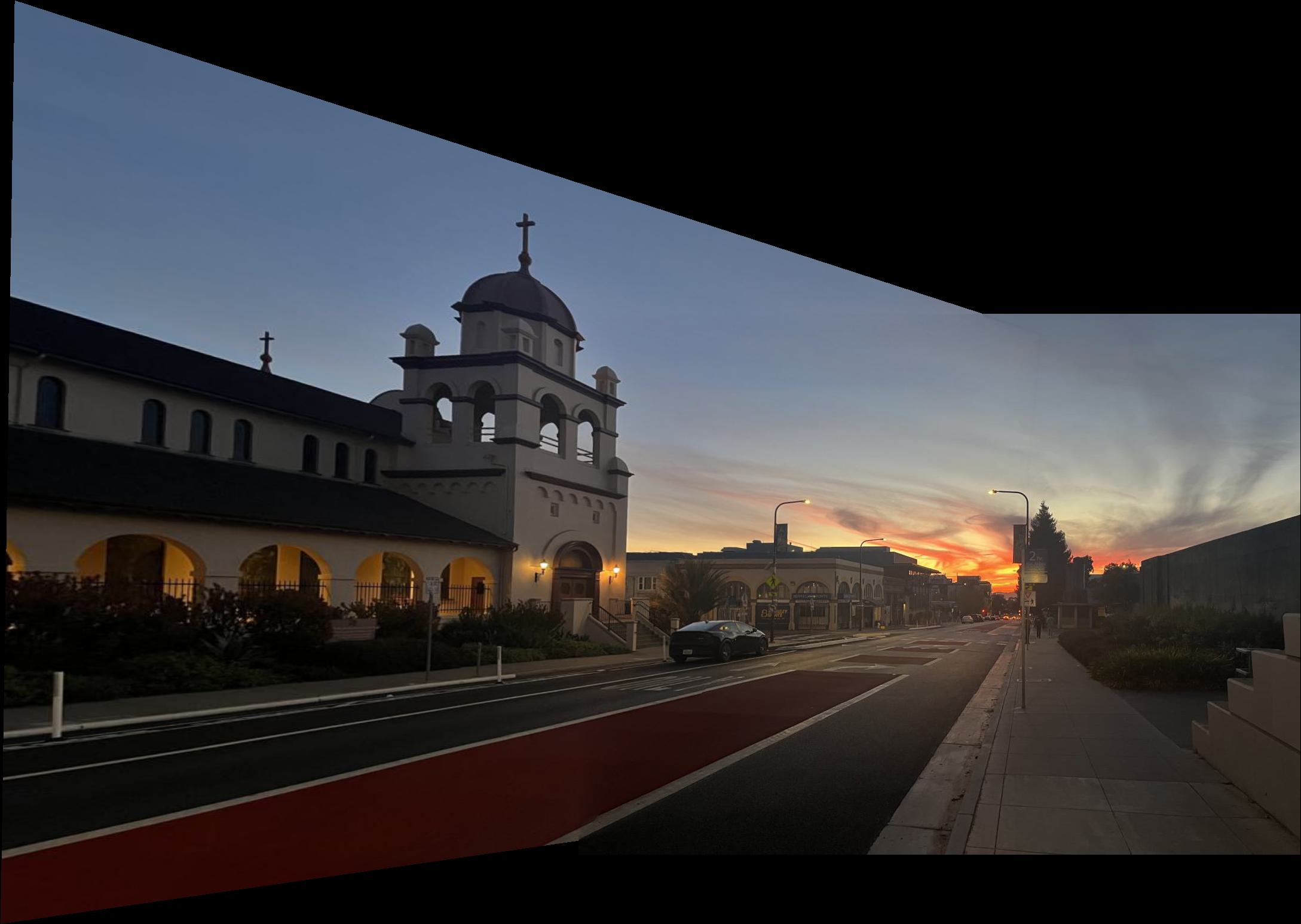
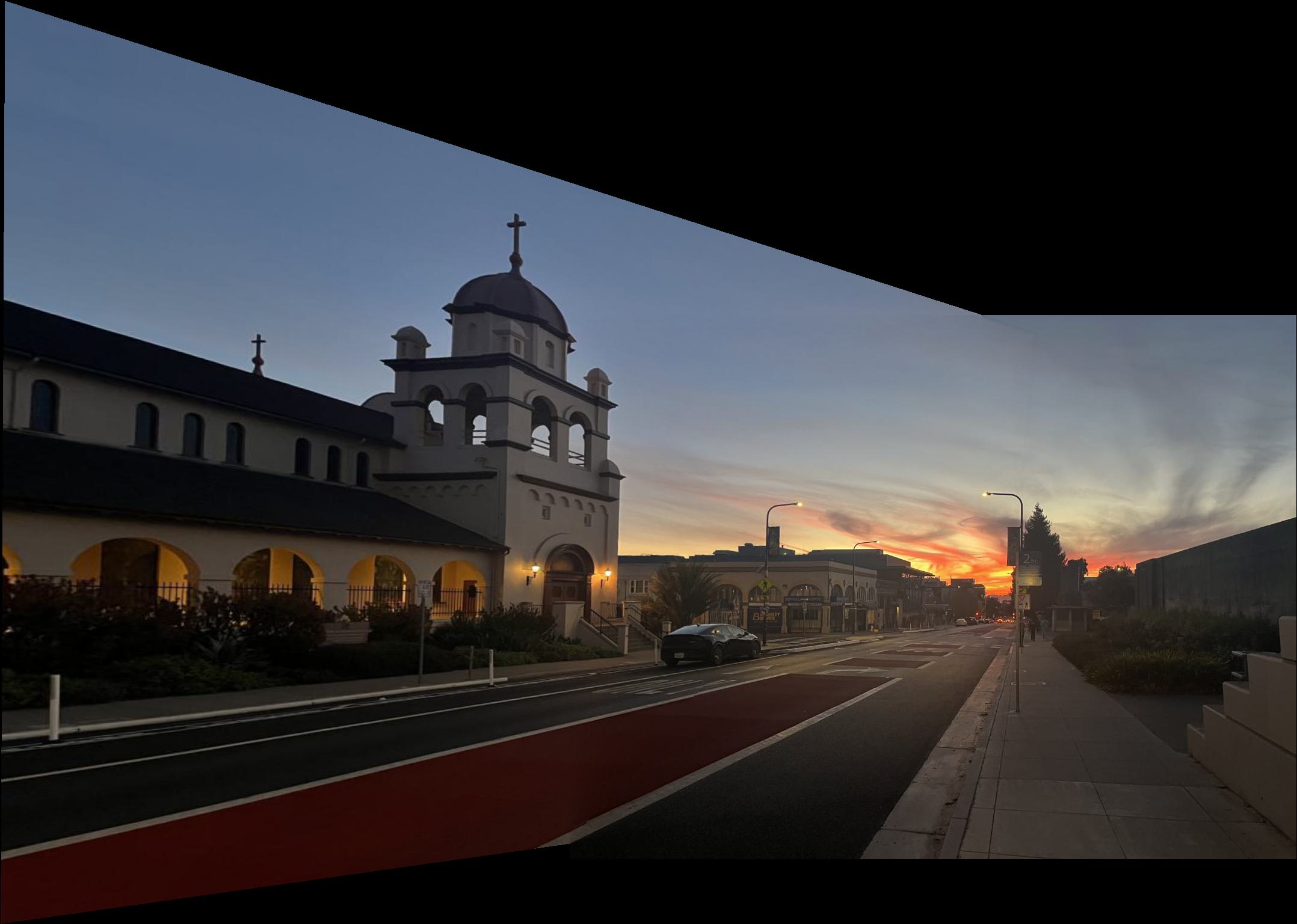
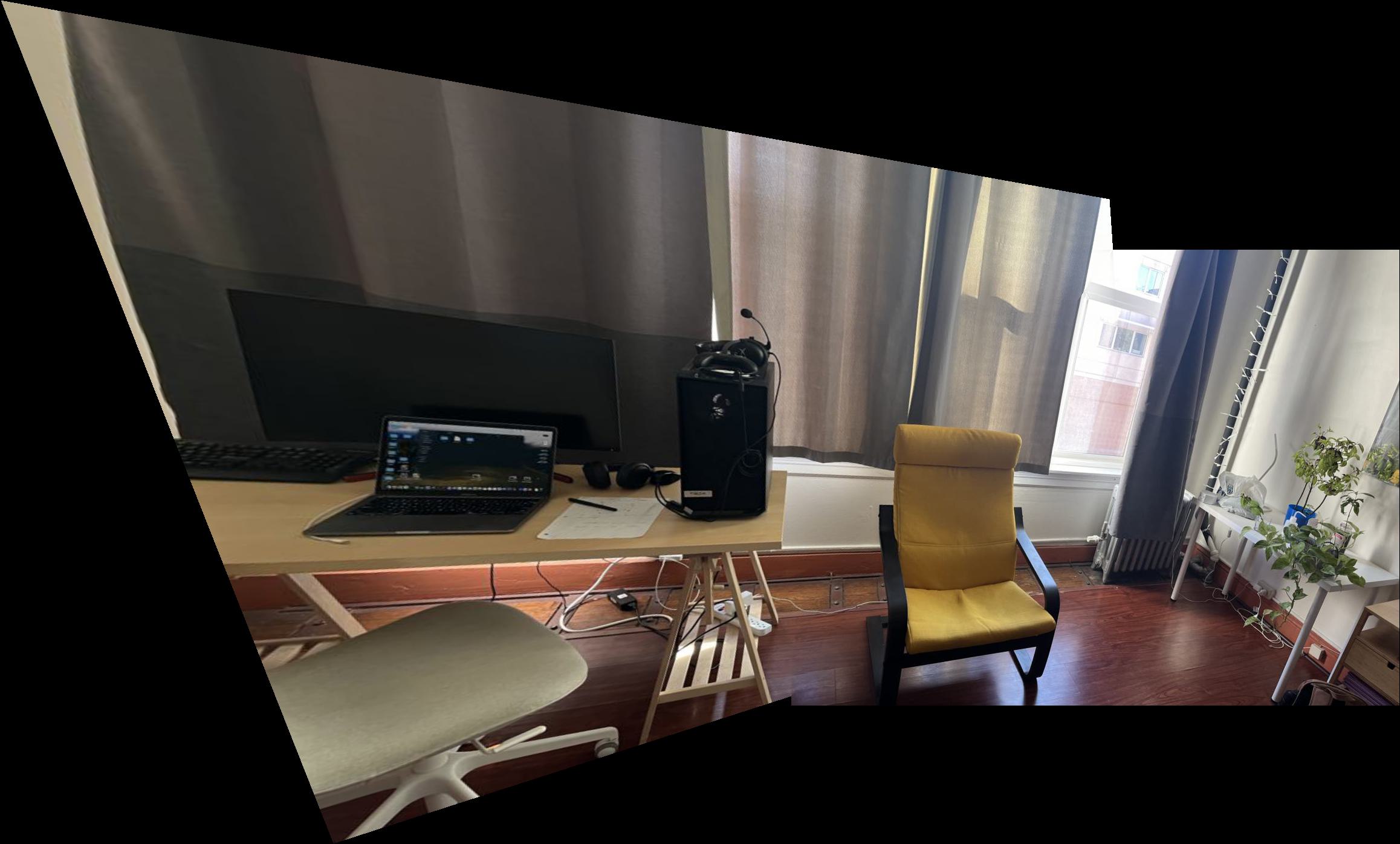
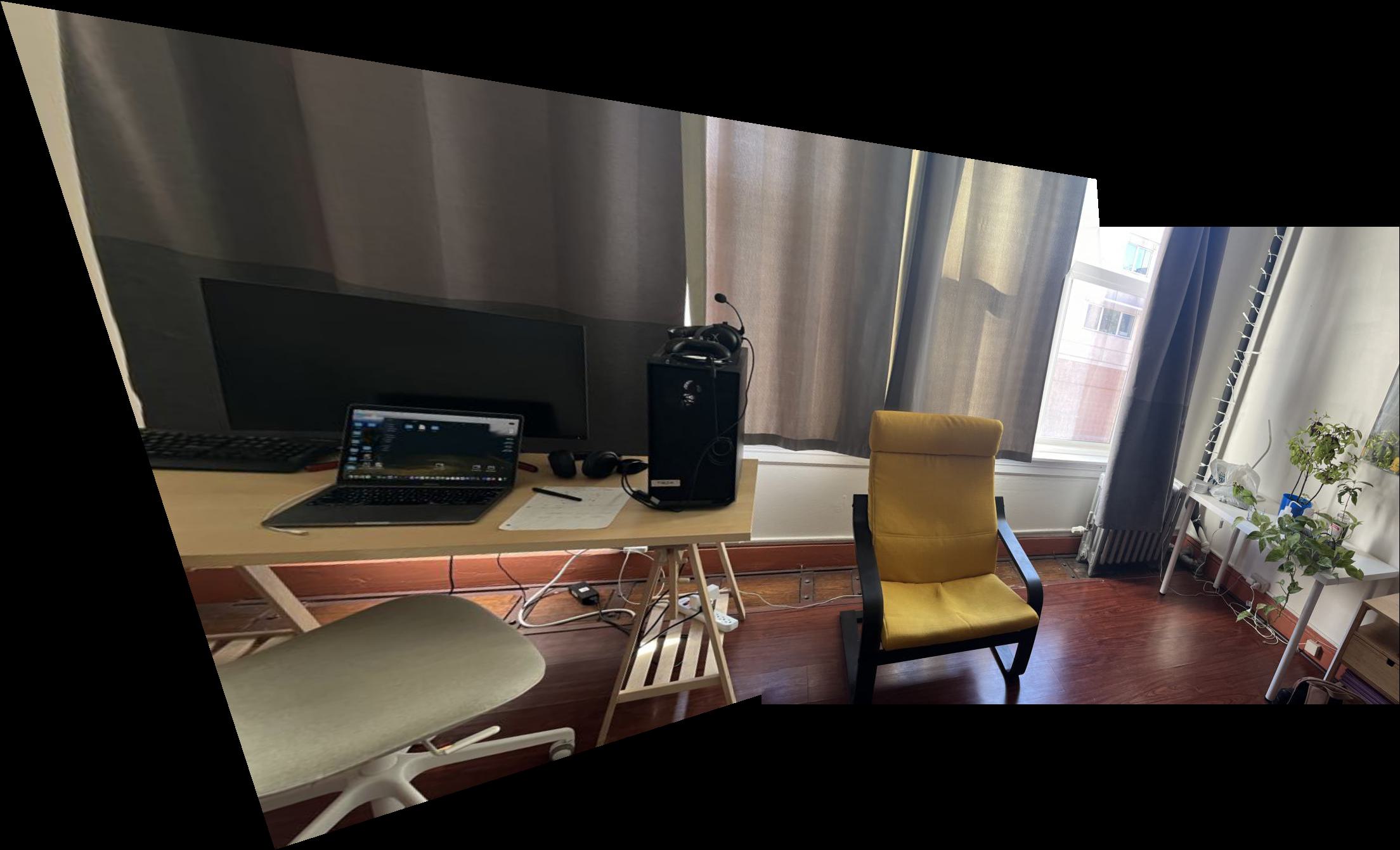
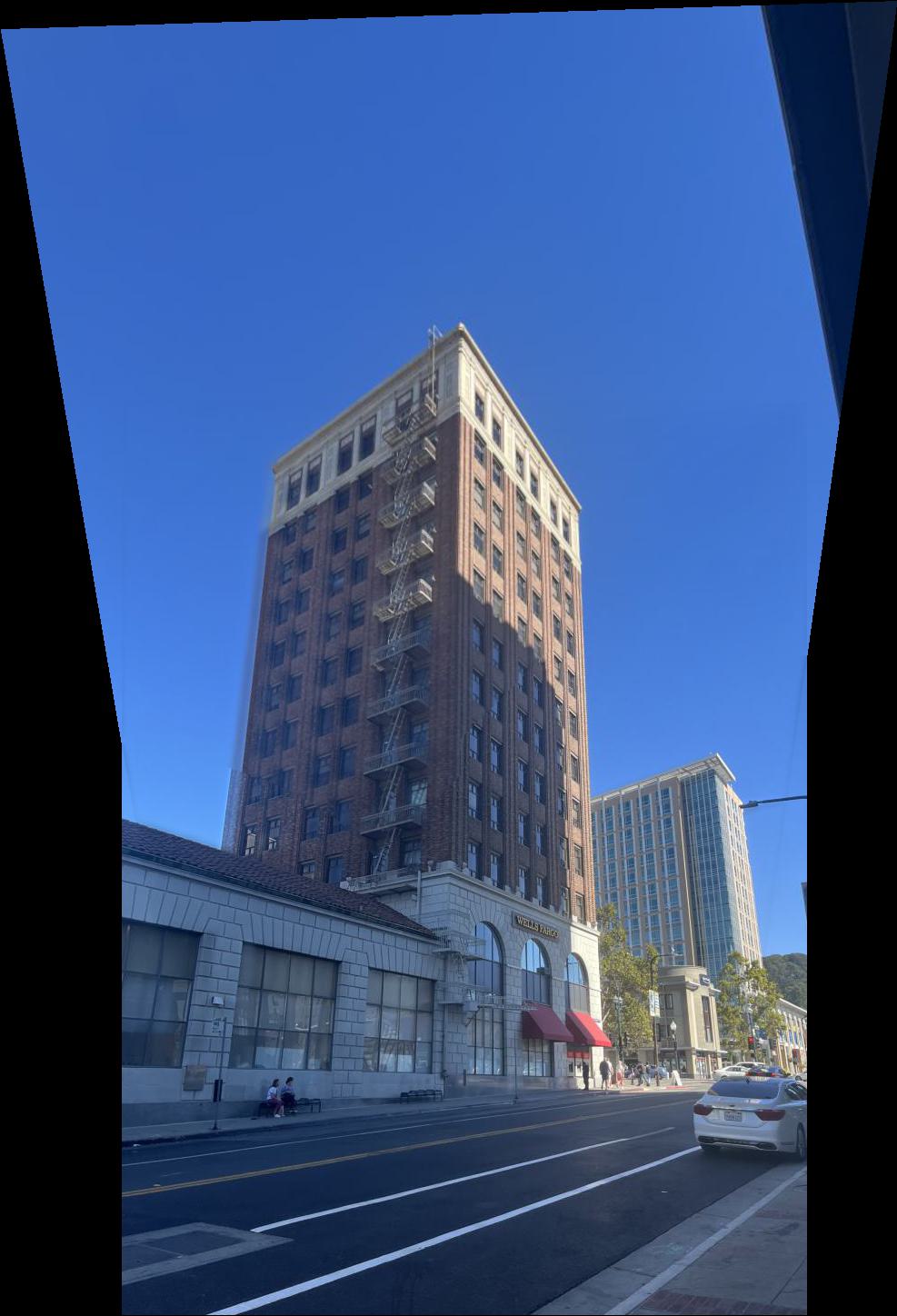
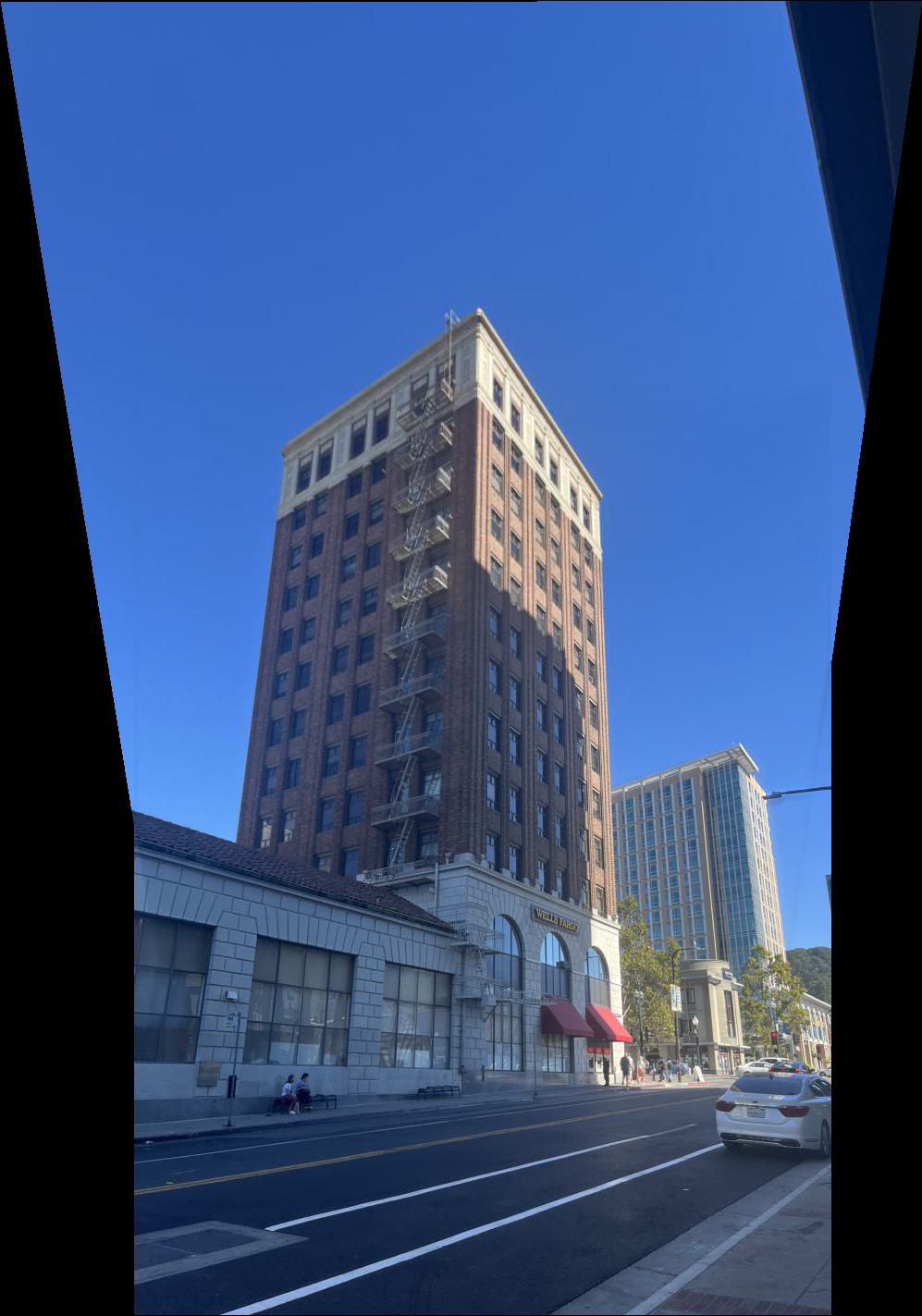
Finally, using the same warping and blending as part A, we can create the mosaics. Below are the results, with the automatically stitched ones on top, and the manual ones below.

What I have learned
My favorite part of this project was definitely part B, as it was much more interesting to do the image stitching automatically. In particular I really like implementing ANMS and RANSAC, as it was a bit challenging at first to understand parts of the paper, but was satisfying once I understood it and successfully implemented the algorithms. Specifically I liked how they both used very simple motivations, obtaining uniformly distributed points and computing a homography that is not sensitive to outliers, and then then used unique ideas to address those.
