By Alex Becker

Part A

Part 0

The first set of images was generated with 20 num_inference_steps

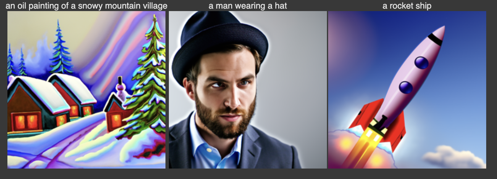
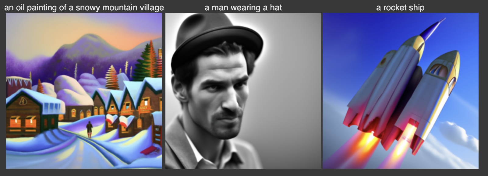
The second set below was generated using just 10, which ran much faster. It’s interesting however because for the oil painting of the snowy mountain village, I think the one with less inference steps actually looks better overall. However, we see that there are a couple unusual things such as the very large piles of snow towards the back. The man arguably looks better with less inference steps, although the picture is in black and white, while the rocket looks pretty strange. It’s less cartoon like than the one with 20 steps, but also looks like a combination of two disfigured rockets.

Part 1: Implementing forward process

For this part we implement the forward process of adding different amounts of noise to the clean source image at different time steps. Here is an example of a clean source image, as well as the image at time steps 250, 500, and 750.

1.2: Classical Denoising

Before actually using a diffusion model, we will first try to denoise the test images above just by using Gaussian blurring. However, we don’t really expect this to work well, as we’re losing so much information as t gets higher and blurring cannot recover what was lost. It can really only smooth small amounts of noise. We see below that there is a tradeoff between reducing the noise and making the image too blurry, depending on how large we make the kernel. As the amount of noise increases, we have to increase the kernel size to try to smooth it, but the image becomes more blurry as a result.

1.3 One-step Denoising

Now we actually use a trained unet to perform one-step denoising. Specifically, we have a unet which has been trained to denoise images, given a timestep and noisy image. The unet estimates the noise added to the original clean image at the given timestep. As we can see below, this does a much better job than the Gaussian blurring, because it at least tries to recover some of the lost information. Even if it isn’t correct, it at least looks like real images.

1.4 Iterative Denoising

We can see that the Unet above did much better than the classical denoising techniques, but as we add more noise it starts to perform poorly. Now, we will implement iterative denoising. However, since our most noised image is at step t=1000, it would be too inefficient to go through every step and denoise. Fortunately, we are able to actually skip over timesteps in strides. In the example below, I started at timestep 990 and took strides of 30. I display the result at every 5th loop of denoising:

Below is the result of single step denoising, as well as gaussian blurring, which look much worse.

1.5: Diffusion Model Sampling

We can also sample by starting with random noise and iteratively denoising. For this we use the prompt “a high quality photo.” Here are 5 examples of sampling.

1.6: Classifier-Free Guidance (CFG)

We can then use classifier free guidance to improve our image quality, as seen below. With CFG, we use both a conditional and unconditional noise estimate.

1.7

Using the SDEdit algorithm, we can “translate” our image by adding noise to it, and then denoising, causing our model to hallucinate something new. Below, we have 3 examples of test images, and results of this translating, starting at different noise levels. If we start at an earlier starting index, we will have more noise meaning the result will be less similar to the original.

Editing hand drawn and web images:

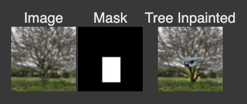
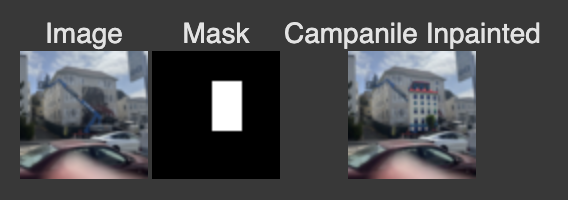
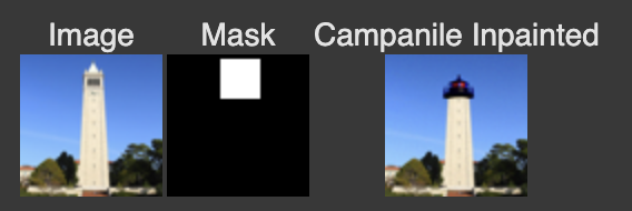
Inpainting

Text-Conditional Image to image translation

This is the same as the previous image translation, except now we use the prompt “a rocket ship”

1.8 Visual Anagrams

To create visual anagrams, during a training step, we denoise an image with one prompt, obtaining our first noise estimate. Then, we flip the image upside down and denoise with a different promp, obtaining a new noise estimate. We can flip this second estimate and average it with the first. Then we perform a denoising diffusion step on this averaged estimate. Below are 3 examples of this.

1.9

We can create image hybrids similar to how we created anagrams, except instead of averaging two noise estimates, we take the high frequencies of one noise estimate and the low frequencies of another. The result is that from far away, the generated image should reflect one prompt, while close up, it should reflect the other prompt.

Part B

In this part of the project we train our own diffusion model on the MNIST dataset

Part 1: Single Step Denoising UNET

In this part, we first implement a UNet and train it to perform one step denoising. To train the model to be able to do this, we just add noise to training images, input these noised images into the implemented Unet, and then optimize of L2 loss of the difference between the original clean image and the resulting “denoised” image that is output by the Unet. We also choose a value sigma which scales the gaussian noise added to each pixel. Below is an example of images noised with different sigma values.

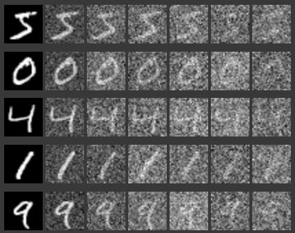
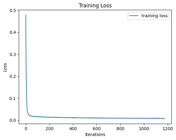
Below are example results of our model’s denoising. The first column is original training images, then noised images, then denoised images with the model being trained for 1 epoch, then denoised images with the model being trained for 5 epochs

While we trained our model with a sigma value of .5, we can also see how it works for other values of sigma. As we would expect, it doesn’t work as well as sigma gets very high. The sigma values used are the same as mentioned above.

Part 2: Training a Diffusion Model

Now, we implement the DDMP paper to use our UNet to iteratively denoise an image. For this step, we make one small change to the model: Before, we were minimizing the loss between the original clean image and our denoised image, while now we minimize the loss between the added noise and the predicted noise. Because we now want to iteratively denoise, we need to somehow condition the model on the timestep of a noised image, meaning how far along the process of denoising it is. To do this we had to add two more components to the UNet architecture, which use fully connected layers to inject time values into the model, so that our model can be conditioned to time.

Now, to train this model, we just have to choose a training image, sample a random t value, and then pass these in to our model. We then repeat this many times and optimize over the L2 loss as explained previously.

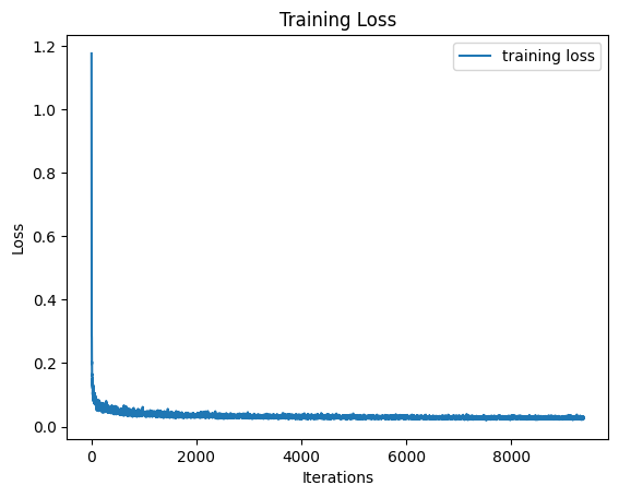
We can also sample from our model now by iteratively denoising generated pure noise. Below are some results of this.

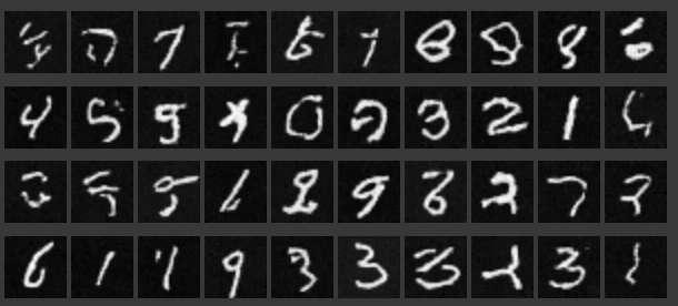
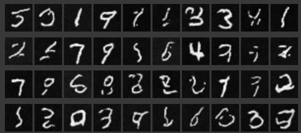
We can see that while some of the sampled images above look pretty, good, many of them don’t look like actual numbers. To improve this, we can also introduce class conditioning, similar to how we previously introduced time conditioning. We just have to add two more fully connected blocks, which this time inject a one-hot encoded vector of a digit class (1-9). This way, when training the model, we can use the label of each training image to create these vectors and inject them into the model. This results in the model being able to be conditioned on class.

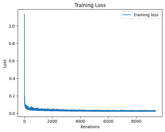
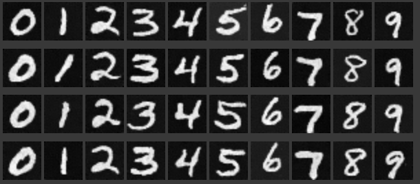
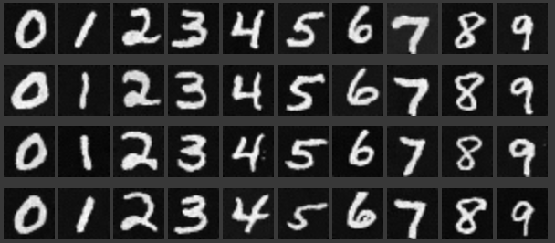
Below are examples of sampling images using this class conditioning