By Alex Becker

Part 1: Fit a Neural Field to a 2D Image

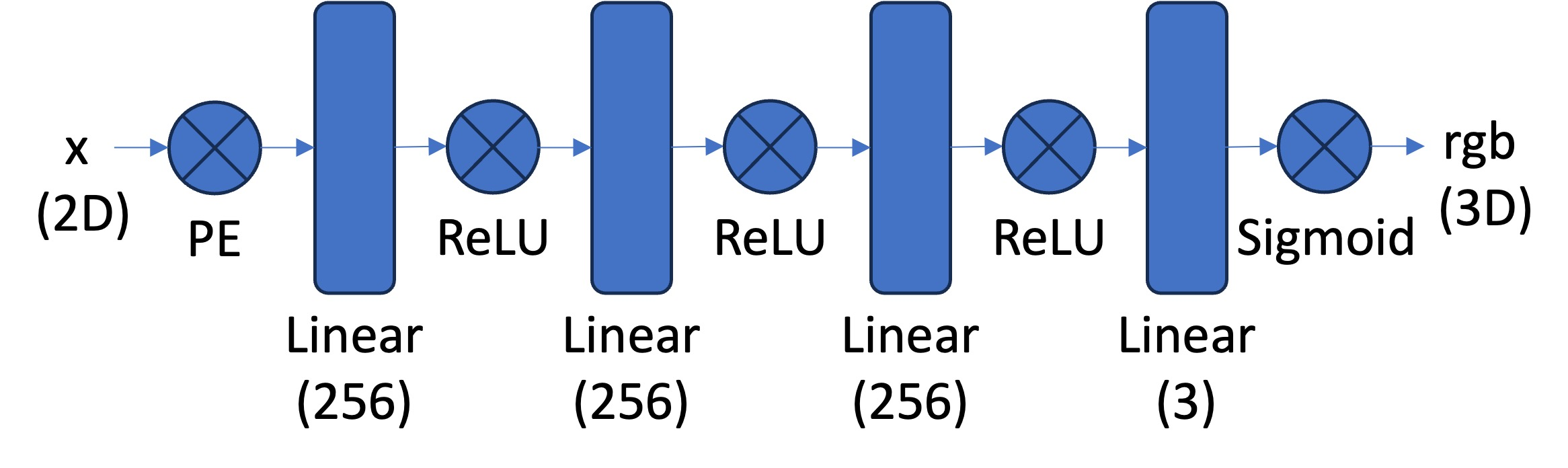
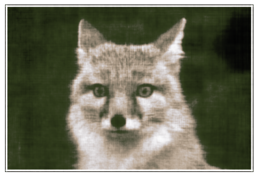
For the architecture of my model, I followed the architecture given in the spec, including a custom sinusoidal positional encoding layer, with a frequency of 10. Therefore, after feeding in the 2D input to this layer, we get a 42D output. For the first training, I just used the suggested hyperparameters: learning rate of 1e-2, same number of layers as the diagram, etc.

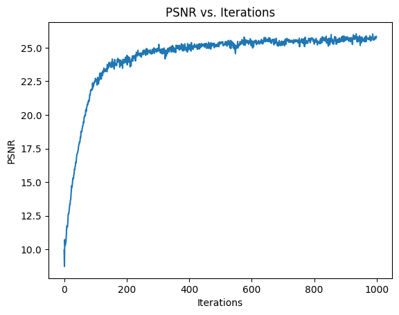
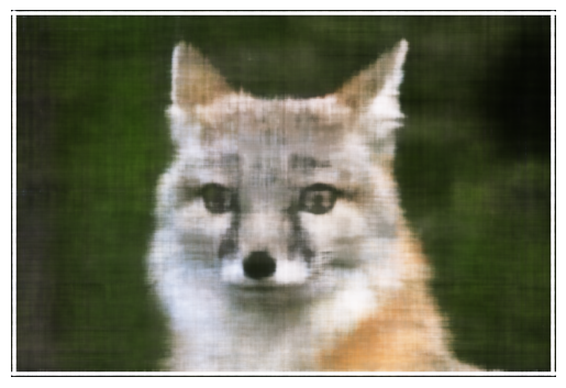
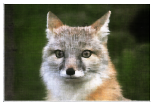
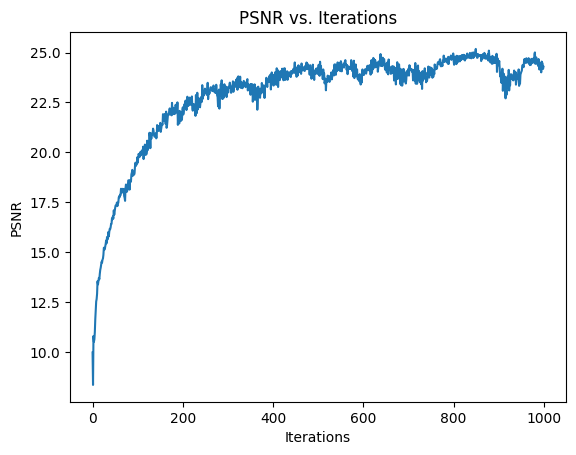
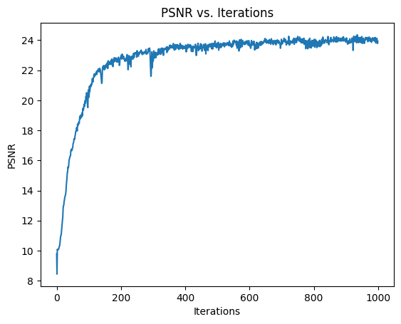
Below is the first image that I trained on, as well as the training PSNR across iterations.

I then tried varying two of the hyperparameters: The learning rate, and adding additional layers to the architecture.

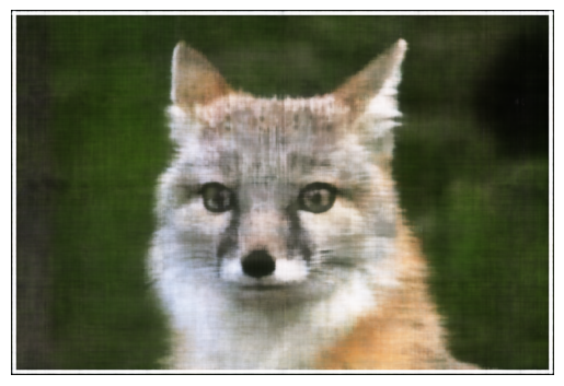
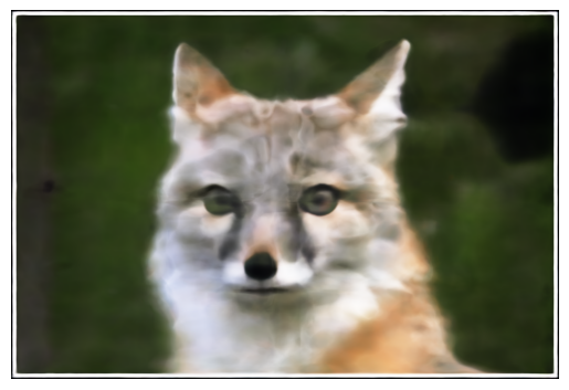
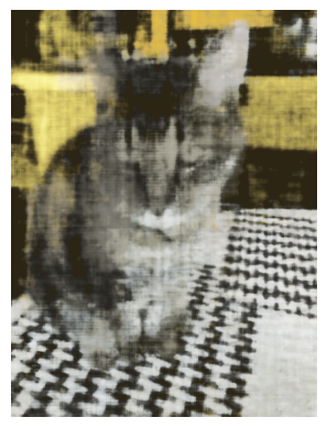
First, I decreased the highest frequency L of the positional encoding to 5 (it was previously 10). Below is the training curve and result after training. We can see that while it reached close to the same PSNR as before, it oscillated a bit as the number of iterations got higher, and the final result doesn’t look quite as good.

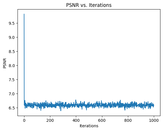
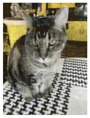
Next, I tried increasing the learning rate to 3e-2 (it was 1e-1 before). We can see from the training curve and result that this learning rate was too high.

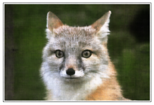
Finally, I tried adding two additional linear + ReLU layers into the architecture. We see that it still doesn’t perform as well as the original architecture, and in particular the entire image has a green hue.

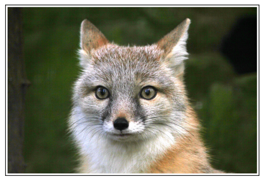
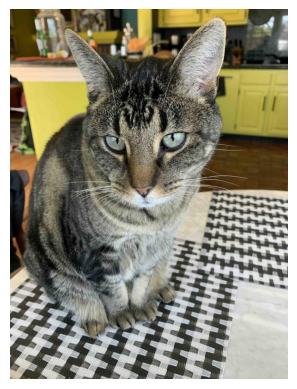
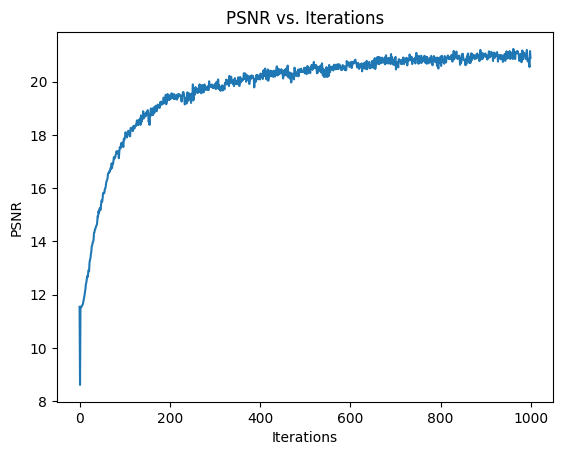
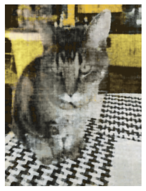
Next, I tried the original architecture, as it seemed to perform the best, on my own image:

Part 2: Fit a Neural Radiance Field from Multi-view Images

Now, we move on to using a neural radiance field and multi-view calibrated images of the Lego scene.

2.1: Create rays from cameras

There are a few steps in order to go from a camera to rays in 3D space. First, starting with a camera, we must covert from the camera’s coordinates to the world coordinates. We are given camera-to-world matrices for each camera, and from this we can extract all the information we need in order to do this conversion. To actually first get to the camera’s coordinates starting with a pixel location, we need to use the intrinsic matrix, K, of the camera. K multiplied by the camera coordinates gives the homogenous pixel coordinates multiplied by s, depth along the optical axis. Finally to make the full conversion from pixel to ray, we need both the ray direction, given by

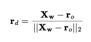
and the ray origin, r_o, which is just the location of the camera, in world coordinates. We can use our previous conversions for this one. I used numpy for all of these conversions.

2.2: Sampling

To sample rays for training, we need to be able get rays from corresponding pixels in the image. Since we implemented the pixel to ray conversion, we can do this. For my implementation, I decided to sample 10,000 rays for each training iteration. I did this by first randomly selecting 20 cameras, and then sampling 10,000 / 20 = 500 pixels coordinates, and then converting those pixels to rays. I did this as I found it simpler to implement than global ray sampling.

Next, since we are working in 3D, we actually have to sample points along each ray. To do this, I uniformly sampled along each ray, adding some noise during training to ensure all points along the rays are trained on. I also used 32 samples per ray.

2.3: Dataloading

In this part, I implemented the actual dataloading described above, to be used to load rays during each training iteration. Additionally, since we are training, we also need to load the actual pixel colors to the corresponding rays, so that we can compute loss to our prediction.

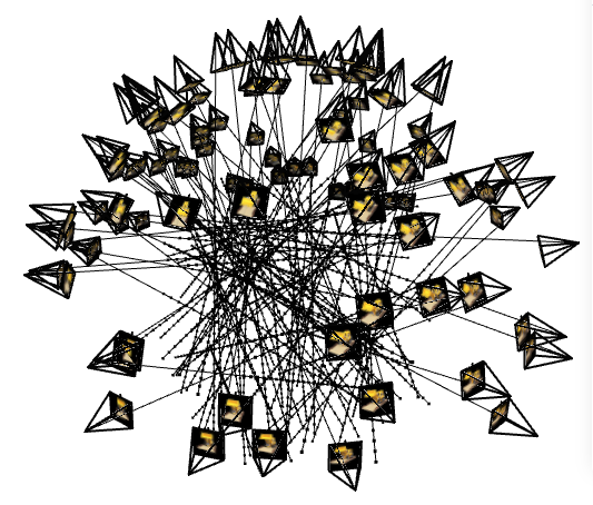
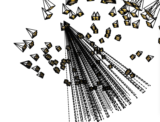
Below is a visualization of the rays and samples (with cameras) on the left. On the right, I’ve made all the rays come from just one camera, to make sure everything looked correct per camera.

2.4: Neural Radiance Field

Now, we actually create the MLP to be used for the Neural radiance field. This is similar to the one used in part 1, except now we have to pass in 3D points, as well as ray directions for the input. Now, the MLP will also output both density and rgb values corresponding to each point. We will then use these for volume rendering. I used the architecture given in the spec:

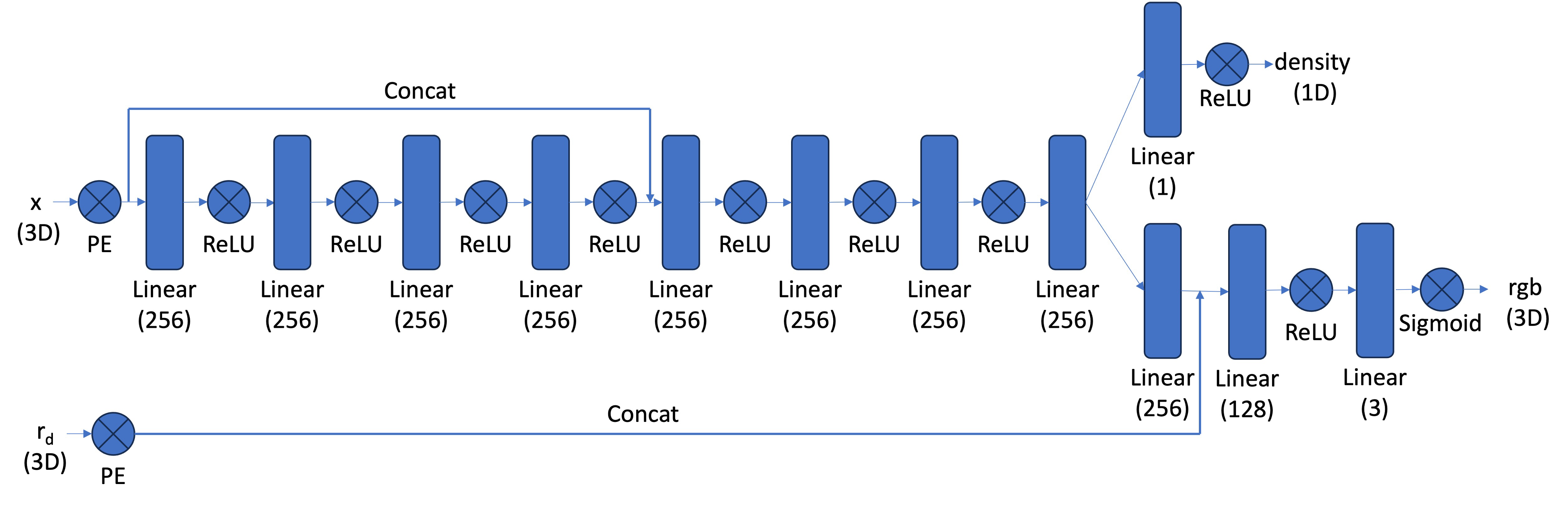
Note that we inject the 3D points (after positional encoding) in a deeper layer, and we also inject the ray direction in a branch of the network that leads to the rgb output. To do this, I just concatenated to the other input using torch. I also used the suggested PE frequencies of L=10 for the points, and L=4 for the ray direction.

2.5: Volume Rendering

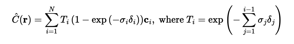
Now, given the output of the MLP, we can actually render an image. The volume rendering equation is given by

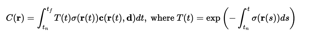
which means that we go along the ray, adding the contribution of infinitesimal intervals to the final color. Obviously, we have to approximate this, given by

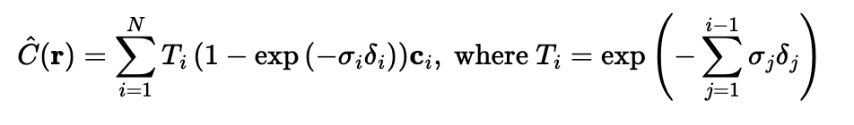
Where the ci is the rgb output of our MLP at sample i, Ti is the probability of the ray not terminating by sample i, and the other term is the probability of the ray terminating at sample i. I used both torch.cumsum and torch.cumprod to do this computation.

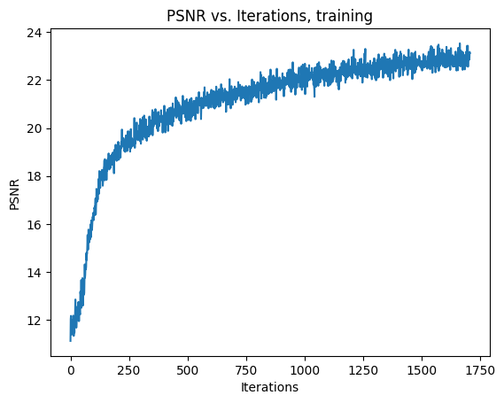
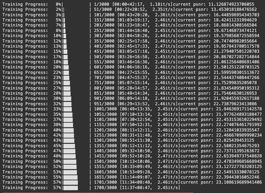
Now, we can train the model. After training for about 1500 iterations, I was able to reach 23 PSNR:

Below, I used my trained network to render novel views according to the provided camera to world test matrices. I then made a gif from the 60 resulting images, which is below.

Bells and Whistles

For bells and whistles, I implemented rendering a background color for the lego video. To do this, I had to modify the previously implemented volrend function. Basically, the goal is to be able to pass in an RGB color, and then the volrend function will output the rendered image as before, but with that RGB color as the background instead of black. To do this we need to modify our implementation of the following equation:

Ti is the probability of a ray not terminating before reaching sample i, which is exactly what happens when for a pixel where we see the background color. It means that its corresponding ray was not terminated. Therefore, we want to use this in our modification. we basically take T_last, the probability of not terminating before the last sample along the ray, multiply it by the chosen color, and add it to the already computed result. Below is an example of the results.